Simulation and survival

In an earlier post we discussed how a survival model was directly equivalent to assuming future lifetime was a random variable.  One consequence of this is that survival models make it quick and simple to simulate a policyholder's future lifetime for the purposes of ICAs and Solvency II.

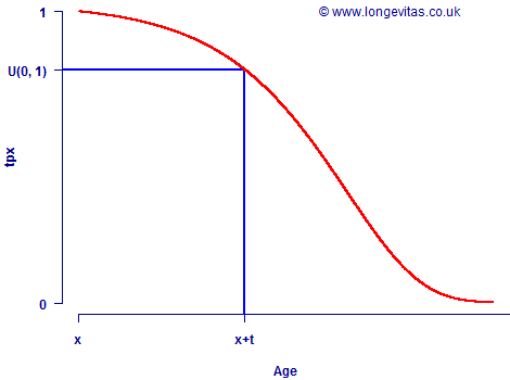
The survival curve is the proportion of lives surviving to each age, i.e. _tp_x in actuarial parlance.  Below is a sample survival curve in red for a life aged x, showing how to read off the probability of survival to age x+t:

For simulation purposes we simply reverse this procedure: we generate a pseudo-random number uniformly distributed over the interval (0, 1), place it on the vertical axis and look up the age at death x+t.

A huge advantage of survival models in simulation lies in the following simple formula for the survival probability:

where H_x(t) is known as the integrated hazard function.  For many survival models H_x(t) has a closed-form expression, and a list for the common actuarial laws of mortality is given in Richards (2008).  The general formula above can then be re-arranged as follows for simulation purposes:

Depending on the choice of mortality law, this formula can be further manipulated to get a direct, closed-form expression for the simulated age at death, x+t.  Using survival models can therefore give a quick and simple way of  simulating the exact age at death from a single U(0,1) variate.  This is particularly efficient when simulating an entire portfolio in run-off, life-by-life, since it means no model points need to be selected.