Don't cut corners
An important class of mortality-projection models is the Cairns-Blake-Dowd (CBD) family. These models are described in a landmark paper by Cairns et al (2009). Three of the most important of the CBD models are M5, M6 and M7, as defined below for age \(x\) and calendar year \(y\):
| M5 | \(\log \mu_{x,y} = \kappa_{0,y} + \kappa_{1,y}S(x)\) |
| M6 | \(\log \mu_{x,y} = \kappa_{0,y} + \kappa_{1,y}S(x) + \gamma_{y-x}\) |
| M7 | \(\log \mu_{x,y} = \kappa_{0,y} + \kappa_{1,y}S(x) + \gamma_{y-x} + \kappa_{2,y}Q(x)\) |
where:
\(\eqalign{S(x) &= \left(x - \bar x\right)\\ Q(x) &= \left(x - \bar x\right)^2-\hat\sigma^2\\ \hat\sigma^2 &= \displaystyle\frac{1}{n_x}\sum_{i=1}^{n_x} (x_i-\bar x)^2}\)
The original CBD definitions were for \({\rm logit\ } q_{x,y}\), but we prefer to work with \(\log \mu_{x,y}\). M5 is essentially a Gompertz law of mortality in each calendar year. M6 is M5 extended to include a cohort term, \(\gamma_{y-x}\). M7 is M6 extended to include an additional quadratic term in age. Iain recently covered some of the issues around fitting and interpreting cohort effects, and an older posting of his looked at forecasting with cohort terms for a mature closed portfolio.
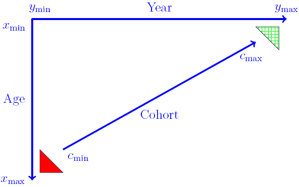
M5, M6 and M7 can be fitted as generalised linear models (GLMs). However, a wrinkle with M6 and M7 (and the APC model) is that cohorts can have widely varying numbers of observations. This is illustrated in Figure 1, where the cohorts in the two triangles have the fewest observations. At its most extreme, the oldest and youngest cohorts have just a single observation each.
Figure 1. Basic data setup.

A direct consequence of this limited data is that any estimated \(\gamma\) term for the corner cohorts will have a very high variance. Cairns et al (2009) dealt with this by simply discarding the data in the triangles in Figure 1, i.e. where a cohort had four or fewer observations. Instead of the oldest cohort having year of birth \(y_{\rm min}-x_{\rm max}\), for example, it becomes \(c_{\rm min}=y_{\rm min}-x_{\rm max}+4\). Similarly, the youngest cohort has year of birth \(c_{\rm max}=y_{\rm max}-x_{\rm min}-4\) instead of \(y_{\rm max}-x_{\rm min}\).
There is a drawback to this approach to fitting cohort effects, namely it makes it harder to compare model fits. We typically use an information criterion to compare models, such as the AIC or BIC. However, this is only valid where the data used are the same. If two models use different data, then their BICs cannot be compared. This would be a problem for comparing the models in Table 1, for example, as the fit for M5 couldn't be compared with the fits for M6 and M7. One approach would be to make the data the same by dropping the corner cohorts for the M5 fit, even though this is technically unnecessary for M5. This sort of thing is not ideal, however, as it involves throwing away data and would have to be applied to all sorts of other non-cohort-containing models.
An alternative approach is to use all the data, but to simply not fit cohort terms in the corners of Figure 1. This would preserve the easy comparability of information criteria between different model fits. To avoid fitting cohort terms where they are too volatile we simply use the M5 formulation in the corners and either M6 or M7 in the rest of the data region. This means that the same data are used, and thus that model fits can be directly compared via the BIC.
References:
Cairns, A. J. G., Blake, D., Dowd, K., Coughlan, G. D., Epstein, D., Ong, A. and Balevich, I. (2009) A quantitative comparison of stochastic mortality models using data from England and Wales and the United States, North American Actuarial Journal, 13(1), 1–35


Add new comment