Visualising covid-19 in experience data

As 2020 edges to a close, life-office actuaries need to set mortality bases for year-end valuations. An obvious question is what impact the covid-19 pandemic has had on the mortality experience of their portfolio? One problem is that traditional actuarial analysis was often done on the basis of annual rates, whereas the initial covid-19 shock was delivered over a period of a couple of months in early 2020 in Europe. Clearly one cannot properly assess the extent of such a short-term shock with annual rates, so what alternatives are available?

In an earlier blog, I defined a non-parametric estimator of short-term patterns in mortality. The first step is to define a non-parametric estimator for the integrated hazard from time \(y\) as follows:

\[ \hat{\Lambda}_y(t) = \sum_{t_i \le t} \frac{d_{y+t_i}}{l_{y+t_i^-}} \qquad (1) \]

where \(t_i\) is one of a set of observed times of death \(\{t_1, t_2, \ldots, t_r\}\) after time \(y\), \(d_{y+t_i}\) lives die at a discrete time \(y+t_i\) and \(l_{y+t_i^-}\) is the number of persons observed alive just before time \(y+t_i\). Equation (1) is the Nelson-Aalen estimator, but applied in time, rather than age. Angus Macdonald wrote a detailed blog on the nature of the Nelson-Aalen estimator.

The second step is to calculate the central difference of \(\hat{\Lambda}_y(t)\) to estimate the mortality hazard, \(\hat\mu_y(t)\), as follows:

\[\hat\mu_y(t) = \frac{1}{c}\left(\hat{\Lambda}_y(t+c/2)-\hat{\Lambda}_y(t-c/2)\right)\qquad(2)\]

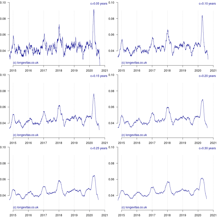
for some smoothing parameter \(c>0\) measured in years. Equation (2) is a uniform kernel smoother and the results for varying values of the bandwidth parameter \(c\) are shown in Figure 1.

Figure 1 shows a rich amount of detail, in part because there is an average of 19 deaths per day and thus a fairly reliable mortality signal even with small values of \(c\). As expected, the non-parametric estimator identifies the seasonal pattern in mortality, especially the winter peaks at the turn of each year. Figure 1 also shows the importance of using an exposure period that balances the number of seasons (there are several options for including seasonal effects in mortality models).

In addition to the usual seasonal patterns, Figure 1 also shows the large covid-19 spike in early 2020; it occurs just as the usual winter excess mortality had passed. With light smoothing (say \(c<0.1\) year) we can see that covid-19 has delivered a shock that is a third higher than the worst winter spike of the past five years:

• In the second week of January 2018 the death rate spiked at 19.6 per 100,000.
• In the first week of April 2020 the death rate spiked at 26.8 per 100,000.

Heavier smoothing (say \(c>0.25\) years) tends to flatten short-term spikes and thus under-state their true peak impact. A value of \(c=1\) year would of course smooth over an entire year, which would mix three months (say) of mortality shock with nine months without, thus flattening the spike even more. This is why using annual rates is not particularly useful when dealing with intense, short-lived shocks, and why actuaries need something more sophisticated than tables of annual \(q_x\) rates.

More details of the estimators in equations (1) and (2) and their application can be found in Richards (2020).

References:

Richards, S. J. (2020) A non-parametric estimator for mortality shocks, working paper, Longevitas Ltd.
Add new comment