Kaplan-Meier for actuaries

In Richards & Macdonald (2024) we advocate that actuaries use the Kaplan-Meier estimate of the survival curve.  This is not just because it is an excellent visual communication tool, but also because it is a particularly useful data-quality check.

One issue is that not all software implementations of the Kaplan-Meier estimate account for left-truncated data.  However, left-truncation is standard in actuarial work, as lives usually only enter observation well into adult life.  To help the actuarial community, Figure 1 shows some R script that calculates the Kaplan-Meier estimate for left-truncated data by age:

Figure 1.  R script for Kaplan-Meier estimates of survival curves with left-truncated data.

################################################################################
#
# Check for updates to this R script at:
#
# https://www.longevitas.co.uk/information-matrix-page/kaplan-meier-actuaries
#
# Read in the data and store as a data frame.
d = read.csv(file="C:/sandpit/SurvivalInput_94729.csv", header=TRUE)
 
# Calculate the exit ages.
d$ExitAge = d$EntryAge + d$TimeObserved
 
# Function to calculate the Kaplan-Meier estimate of the survival curve, tpx.
# Arguments:
#   - g is the data frame, which can be a sub-group, and
#   - i is the interest rate for annuity calculation, e.g. 0.03 for 3%.
# The function returns:
#   - the outset age (x),
#   - the vector Kaplan-Meier estimate (tpx),
#   - the vector of outset age and death ages (ages),
#   - the complete life expectancy from outset (ex), and
#   - the annuity factor for continuous payment of 1 per annum (ax).
KaplanMeier = function(g, i=0)
{
  # Find outset age.
  x = min(g$EntryAge)
  
  # Find ordered set of unique death ages.
  deathages = as.matrix(sort(unique(g$ExitAge["DEATH"==g$Status])))
   
  # Count deaths at each unique death age.
  deaths = apply(deathages, 1, function(y) sum(y==g$ExitAge & "DEATH"==g$Status))
   
  # Count lives in-force immediately prior to each unique death age.
  lives = apply(deathages, 1, function(y) sum(g$EntryAge<=y & g$ExitAge>=y))

  # Calculate Kaplan-Meier estimate of survival curve
  tpx = c(1, cumprod(1-deaths/lives))
  ages = c(x, deathages)
  # Calculate crude life expectancy and annuity factor.
  dx = c(diff(ages),0)
  ex = sum(dx*tpx)
  ax = sum(dx*tpx*(1.0+i)^(x-ages))
   
  return(list(ages=ages, x=x, tpx=tpx, ex=ex, ax=ax))
}
 
# Calculate separate Kaplan-Meier estimates for males and females.
Females = KaplanMeier(d["F"==d$Gender,], 0.03)
Males = KaplanMeier(d["M"==d$Gender,], 0.03)
 
# Function to format legend label.
label = function(title, KM)
{
  return(bquote(.(title)~e[.(KM$x)]==.(sprintf("%.2f", KM$ex))))
}
# Plot the Kaplan-Meier step functions.
plot(Females$ages, Females$tpx, type="S", main="Kaplan-Meier estimate",
     xlab="Age", ylab="Survival probability", col="red", lwd=2)
lines(Males$ages, Males$tpx, type="S", col="blue", lwd=2)
legend("topright", col=c("red", "blue"), lty=c(1, 1), lwd=c(2, 2), bty="n",
       legend=c(label("Females", Females), label("Males", Males)), cex=1.5)
################################################################################

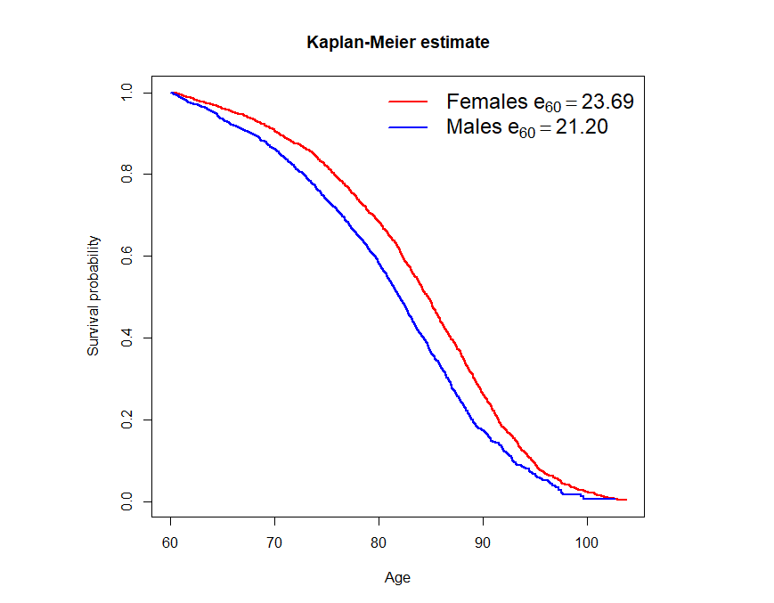
Readers can scrape the R script in Figure 1 and use it directly with Longevitas input files (but remember to change the filename!).  For those without access to Longevitas, see the example file on the right. After running the script on the example file, you should get something like Figure 2 in your R console:

Figure 2.  Kaplan-Meier estimates of the survival curves for males and females.

References:

Macdonald, A. S., Richards. S. J. and Currie, I. D. (2018). Modelling Mortality with Actuarial Applications. Cambridge University Press, Cambridge.
Richards, S. J. and Macdonald, A. S. (2024) On contemporary mortality models for actuarial use I: practice, British Actuarial Journal (to appear).
Kaplan-Meier in Longevitas
Longevitas will generate Kaplan-Meier estimates for each sub-group when you set the option in the Advanced Options section of the initial modelling screen.
Longevitas automatically deduplicates portfolio records, and calculates the exposure for each record, taking into account left-truncation and right-censoring.
Example file
SurvivalInput_94729.csv contains example scheme data prepared in accordance with the steps described in Macdonald et al (2018, Chapter 2), including validation and deduplication. For the purposes of the R script on the left, the key fields are:
EntryAge, which contains the (left-truncated) entry age in years,TimeObserved, which contains the time in years until death or censoring, andStatus, which contains "DEATH" for a death, or 0 for a censored observation.
Previous posts
Actively Beneficial?
How should we describe a lifestyle change that doubles our likelihood of suffering a major traffic accident? Oddly, evidence from Scotland suggests the answer is "worth making". Let me explain.
When is your Poisson model not a Poisson model?
The short answer for mortality work is that your Poisson model is never truly Poisson. The longer answer is that the true distribution has a similar likelihood, so you will get the same answer from treating it like Poisson. Your model is pseudo-Poisson, but not actually Poisson.
Add new comment