Functions of a random variable

Assume we have a random variable, \(X\), with expected value \(\eta\) and variance \(\sigma^2\). Often we find ourselves wanting to know the expected value and variance of a function of that random variable, \(f(X)\). Fortunately there are some workable approximations involving only \(\eta\), \(\sigma^2\) and the derivatives of \(f\). In both cases we make use of a Taylor-series expansion of \(f(X)\) around \(\eta\):

\[f(X)=\sum_{n=0}^\infty \frac{f^{(n)}(\eta)}{n!}(X-\eta)^n\]

where \(f^{(n)}\) denotes the \(n^{\rm th}\) derivative of \(f\) with respect to \(X\). For the expected value of \(f(X)\) we then have the following second-order approximation:

\[{\rm E}[f(X)] \approx f(\eta)+\frac{f''(\eta)}{2}\sigma^2\qquad(1)\]

where \(f''\) denotes the second derivative of \(f\). For a first-order approximation we would just use \({\rm E}[f(X)]\approx f(\eta)\).

For the variance of \(f(X)\) we have the following first-order approximation (also known as the delta method):

\[{\rm Var}[f(X)] \approx [f'(\eta)]^2\sigma^2\qquad(2)\]

where \(f'\) denotes the first derivative of \(f\). Clearly, the approximation in equation (2) leads to a simple formula for the standard error (se):

\[{\rm se}[f(X)] \approx |f'(\eta)|\sigma.\qquad(3)\]

A more accurate approximation for the variance of \(f(X)\) could be obtained using the second-order approximation:

\[{\rm Var}[f(X)] \approx [f'(\eta)]^2\sigma^2-\frac{[f''(\eta)]^2}{4}\sigma^4.\qquad(4)\]

How much of a difference is there between equations (2) and (4) in practice? To illustrate this we will consider a transformation sometimes used in mortality work, namely the logarithm of the logistic function:

\[f(x) = x-\log\left(1+e^x\right)\qquad(5)\]

which has the following first and second derivatives:

\begin{eqnarray} f'(x) &=& \frac{1}{1+e^x}\\f''(x) &=& \frac{-e^x}{(1+e^x)^2}.\end{eqnarray}

Where does this particular definition of \(f\) come from? Well, a GLM for mortality using a Poisson error and a log link is such that the logarithm of the fitted mortality rate is just the linear predictor, \(\eta\). If we use a logit link, however, the logarithm of the fitted mortality rate is given by the function \(f\) defined above in equation (5). If we were working on a logarithmic scale, the function \(f\) is then what we would use to compare the fitted rates from a logit-link GLM with the fitted rates from a log-link GLM.

Back to our two approximations. We now have the following second-order approximations:

\begin{eqnarray}{\rm E}[f(X)] &\approx& \eta-\log\left(1+e^\eta\right)-\frac{e^\eta\sigma^2}{2\left(1+e^\eta\right)^2}\qquad(6)\\{\rm Var}[f(X)] &\approx& \frac{\sigma^2}{(1+e^\eta)^2}\left[1-\frac{e^{2\eta}\sigma^2}{4(1+e^\eta)^2}\right]\qquad(7)\\{\rm se}[f(X)] &\approx& \frac{\sigma}{1+e^\eta}\sqrt{1-\frac{e^{2\eta}\sigma^2}{4(1+e^\eta)^2}}.\qquad(8)\end{eqnarray}

What is the difference between approximations (3) and (8) in practice? Figure 1 below shows an example of the ratio of the standard error according to (3) relative to the standard error according to (8).

Figure 1. Ratio of standard errors approximated with equations (3) and (8). Source: own calculations using CBD5 Perks model applied to mortality data from ONS for males in England & Wales, ages 50–104, 1971–2015.

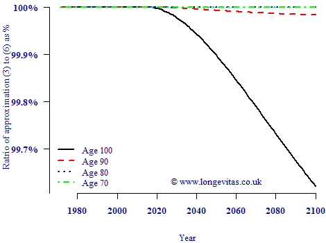
Figure 1 shows that there is no meaningful difference between the first- and second-order approximations for \({\rm se}[\log\mu]\) in the region of the data. Even in the forecast region the approximations are very close, with the largest error at the oldest ages and the longest term being 0.5% at worst. In terms of accuracy of the standard error it doesn't matter in this instance whether we use a first- or second-order approximation.